In large-scale storage systems, erasure codes are essential for reducing storage costs and maintaining high durability. Erasure codes can also be used in more creative ways, such as reducing network latency by hedging requests 1. There are also many constraints to consider when choosing specific codes such as how often you need to perform repairs, available network capacity, data center redundancy needs, and durability guarantees.
In this post, we build up from simple linear systems in order to build the foundations for Reed-Solomon style codes and using tiny Python snippets along the way. We’ll also keep dependencies minimal and only use NumPy.
We’ll use this notation throughout:
k: data shards per stripem: parity shards per stripen = k + m: total shards per stripe
Storage overhead is n / k, the total shards over the data shards. For example, RS
10+4 means k = 10, m = 4, has 1.4x overhead, and tolerates any 4 shard
erasures. By comparison, 3x replication has 3x overhead and
tolerates 2 replica losses. Placement across disks, nodes, racks, and zones
determines whether those shard losses are truly independent. Some modern codes
intentionally add a bit more parity to reduce repair bandwidth. For example,
locally repairable codes 2.
Here’s a quick comparison:
| Scheme | Overhead | Stripe erasure tolerance | Data read to repair 1 lost shard |
|---|---|---|---|
| 3x replication | 3.0x | 2 losses | 1 shard |
| RS 10+4 | 1.4x | 4 losses | 10 shards |
| RS 12+2 | 1.17x | 2 losses | 12 shards |
Warmup: solving a linear system Link to heading
A linear equation in two variables looks like:
$$ 2x + 3y = 7 $$
Two independent equations define a single point (x, y).
For example:
$$ 2x + 3y = 7 \\ x - y = 1 $$
You can solve this by hand, but it is also just a matrix equation:
$$ A c = b $$
where A is the coefficient matrix, c is the unknowns, and b is the
result vector.
Here is a tiny NumPy example:
|
|
Same idea, same tooling, if you move from 2 variables to 3+ variables.
A polynomial view Link to heading
Okay, here is where the ’trick’ comes in. The key is to encode data as coefficients of a polynomial. For example:
$$ M(x) = 2 + 3x + 4x^2 $$
The coefficients [2, 3, 4] are the data. If we evaluate M(x) at multiple
points, we get more equations than unknowns, which gives redundancy.
This is the idea behind Reed-Solomon codes 3.
Encoding by evaluation Link to heading
We will:
- Define a message polynomial.
- Evaluate it at 5 points to create the codeword.
- Lose two points and recover the coefficients from the remaining points.
1) Define the message polynomial Link to heading
Let:
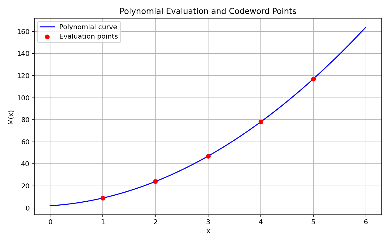
$$ M(x) = 2 + 3x + 4x^2 $$
The coefficients [2, 3, 4] are the data.
|
|
2) Choose evaluation points Link to heading
We will use 5 distinct points: 1, 2, 3, 4, 5.
|
|
3) Encode: evaluate the polynomial Link to heading
We use Horner’s method to evaluate the polynomial (at the given points) and generate the codeword, which is just the list of outputs at those points. It’s a fast, standard way to evaluate polynomials.
|
|
4) Plot the polynomial and points (optional) Link to heading
This part is optional, but we can plot the polynomial at the different selected points in order to visualize what we’re doing.
|
|
5) Simulate erasures Link to heading
In this example, we simulate two erasures at indices 1 and 3 (that is,
x = 2 and x = 4). Assume we only receive evaluations at indices 0, 2, 4.
|
|
6) Recover the polynomial Link to heading
To recover the coefficients, we write the equations in matrix form. A
Vandermonde matrix is just the table of powers of the x-values (1, x, x^2, ...)
so that A * coeffs = y. Solving that system gives us the original
coefficients.
If there is a unique solution, then the matrix A must be invertible. That
means we can do:
$$ coeffs = A^{-1} y $$
In our example, that means we can solve for the unknowns in one step. The x-values must be distinct for this to work.
Where do the linear equations come from? Pick an x, plug it into the
polynomial, and you get an equation like:
$$ c_0 + c_1 x + c_2 x^2 = y $$
The unknowns are the coefficients c0, c1, c2, .... If there are k
coefficients, you need at least k distinct equations (i.e., k different
x values) to solve for them. The encoder’s job is to pick distinct x values,
evaluate the polynomial, and send those outputs (the codeword).
|
|
Two erasure examples:
- Lose two points (keep indices 0, 2, 4). This is the example above.
- Lose two different points (keep indices 1, 2, 3). This also works because we still have 3 distinct points.
The rule is simple: a degree-2 polynomial needs any 3 distinct points.
This is exactly the erasure model: we lose symbols, but we know which ones.
Erasure vs. error correction (quick note): erasures mean we know which symbols are missing, while errors mean unknown symbols might be wrong. This post only covers erasures.
From linear equations to Reed-Solomon Link to heading
Reed-Solomon codes are polynomial evaluation codes over a finite field.
They are MDS (maximum distance separable): any k out of n symbols recover
the original data.
The encoder chooses k data symbols (the coefficients) and outputs n evaluated
symbols. Any k of those n are enough to reconstruct the polynomial, so you
can tolerate n - k erasures.
Key point: the decoder is just solving a linear system.
Finite fields (Galois fields) Link to heading
The example above used real numbers, but storage systems use finite fields so that all arithmetic stays within a fixed symbol size (like a byte).
A Galois field GF(2^m) has exactly 2^m elements. Arithmetic wraps around inside
this field, so every non-zero element has a multiplicative inverse, and all
linear systems behave nicely for coding.
In practice, many Reed-Solomon deployments use GF(2^8) for byte symbols, though other symbol sizes are also used. The same linear algebra applies, but the math is done modulo a field polynomial instead of with reals.
If you want a tiny bit-level multiplication example in GF(2^3), see the appendix at the end.
A simple erasure code end-to-end Link to heading
Let k = 3 data symbols d0, d1, d2. We create n = 5 encoded symbols by
choosing 5 distinct points and evaluating the polynomial:
$$ M(x) = d_0 + d_1 x + d_2 x^2 $$
The encoder sends M(1), M(2), M(3), M(4), M(5).
If any two are erased, the decoder picks any 3 remaining points, builds the
Vandermonde matrix, and solves for [d0, d1, d2].
That is the entire idea: erasure codes are linear equations plus redundancy.
A full “hello” example (recover the original string) Link to heading
Okay, our equivalent “hello” test will tie all these concepts together. Here is
a minimal example that encodes the string "hello", then simulates losing some
encoded symbols and recovers the original string by solving for the coefficients
again.
We will use a degree-4 polynomial code over the integers. We treat the bytes as
the polynomial coefficients, evaluate it at x = 1..7, and use the extra points
as parity. This is still a toy example (not a true
Reed-Solomon over a finite field), but the mechanics are the same.
|
|
Warning: this demo uses floating point + rounding, which is not exact. Real Reed-Solomon uses finite field arithmetic so every step is exact and stays in a fixed-width byte.
What matters in distributed storage Link to heading
If you are onboarding to erasure coding for storage systems, these are usually the practical design levers:
-
Stripe geometry (
k + m).
You split each stripe intokdata shards andmparity shards. -
Storage overhead.
Overhead is(k + m) / k. -
Fault tolerance.
You can tolerate up tomshard erasures per stripe (assuming shard placement avoids correlated failures). -
Repair bandwidth.
In classic Reed-Solomon, repairing one lost shard usually readsksurviving shards. This is where local-repair codes can help. -
Write/read amplification.
Small random writes often force read-modify-write work for parity updates.
This is why production systems choose codes based on more than durability: repair speed, network cost, and placement constraints often dominate.
Closing Link to heading
This is the simplest path from linear equations to Reed-Solomon. Of course, there is a lot that we did not cover and many ways to approach this subject, but this path is often approachable for people with limited exposure to linear algebra. In a follow-up, we can explore other families of error-correcting codes.
Appendix: optional GF(2^3) multiplication Link to heading
This is a tiny bit-level example. It is optional, and only here if you want to see what finite-field multiplication can look like in code.
|
|
If you want to suggest edits or improvements, feel free to open a pull request in the source repository 4.
References Link to heading
- M. Brooker, “Erasure Coding versus Tail Latency,” Jan. 6, 2023. https://brooker.co.za/blog/2023/01/06/erasure.html
- C. Huang et al., “Erasure Coding in Windows Azure Storage,” USENIX ATC, 2012. https://www.usenix.org/system/files/conference/atc12/atc12-final181_0.pdf
- I. S. Reed and G. Solomon, “Polynomial Codes over Certain Finite Fields,” Journal of the Society for Industrial and Applied Mathematics, vol. 8, no. 2, pp. 300-304, 1960. DOI: https://sites.math.rutgers.edu/~zeilberg/akherim/ReedS1960.pdf
- Source file for this post: https://github.com/tallwater/agriel-blog/blob/main/agriel-blog/content/posts/erasure-codes-basics.md